Direction Finding Theory#
Angle estimation (direction-finding) methods and antenna arrays are essential for the positioning system to work properly. The history of direction finding theory goes back more than 100 years, when the first attempts to solve this problem were made using directional antennas and, obviously, purely analog systems. In the years following, test methods moved to the digital world, but the basic principles are still similar. These direction-finding methods are already used in many applications, such as medical equipment, security, and military devices. This section discusses the basics of some typical antenna arrays and estimation algorithms. In this document direction finding refers to the general problem of estimating arrival and departure angles.
Antenna Arrays#
Antenna arrays for direction finding are usually divided into categories. The most common ones discussed here are Uniform Linear Array (ULA), Uniform Rectangular Array (URA), and Uniform Circular Array (UCA). The linear array is a one-dimensional array, meaning that all the antennas in the array lie on a single line, whereas the rectangular and circular arrays are two-dimensional (2D) arrays, meaning that the antennas are spread in two dimensions (on a plane).
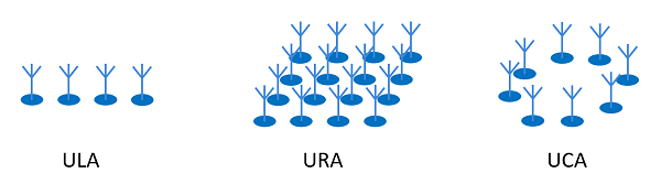
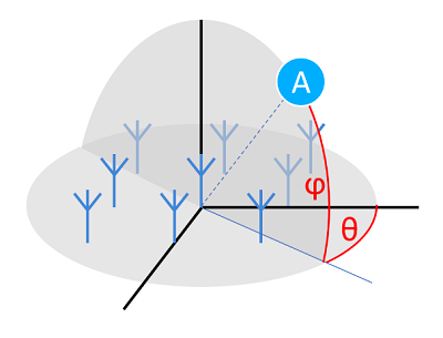
By using a one-dimensional antenna array, one can reliably measure only the azimuth angle, assuming the tracked device moves consistently on the same plane. Also, the azimuth measurement is limited to a 180 degree-wide angle range due to symmetry reasons. With two-dimensional arrays, one can reliably measure both azimuth (theta) and elevation (phi) angles in the 3D half-space, as shown in the following figure. If the array is extended to a full 3D array (antennas spread on all three Cartesian coordinates), then it is possible to measure the full 3D space.
Designing an antenna array for direction finding is not a straightforward task. When antennas are placed in an array, they start affecting each other’s responses; called mutual coupling. Another consideration is that, in most cases, the polarization of the transmitting end cannot be controlled. This creates an additional challenge for the designer. In IoT applications, the devices are often expected to be small and even to work in very high frequency bands. Estimation algorithms often require certain properties from the array. For example, the estimation algorithm called ESPRIT works on the mathematical assumption that the array is divided into two identical subarrays (see Z. Chen, G. Gokeda, Y. Yu, Introduction to Direction-of-Arrival Estimation, Artech House, 2010).
Angle Estimation Algorithms#
Consider the mathematical/algorithmic problem of estimating the angle of arrival based on the input IQ-data. The problem definition itself is simple: estimate the arrival angle of an emitted (narrowband) signal arriving at the receiving array. While the problem statement sounds trivial and a trivial solution is possible, a robust solution for this problem that works in real life is not easy and can require much processing power from the hardware. This section describes the trivial solution, and then provides a high-level overview of two different, more robust, approaches for solving this problem. The first one is basic and called a classical beamformer. The second is a more advanced technique called Multiple Signal Classification (MUSIC). Deeper studies of these estimation algorithms can be found in H. Krim, M. Viberg, “Two Decades of Array Signal Processing”, IEEE Signal Processing Magazine, July 1996, pp. 67-94, and Y.-M. Chen, “On Spatial Smoothing for Two-Dimensional Direction-of-Arrival Estimation of Coherent Signals”, IEEE Transactions on Signal Processing, Vol. 45, No. 7, July 1997.
The Trivial Solution#
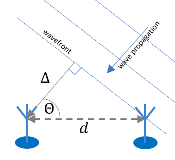
Assume the use of two receiver antennas. If the incoming signal hits these antennas with an oblique incident angle, it results in a phase difference (ψ), because the wavefront propagates with the speed of light (c), and it needs more time to reach the further antenna. Since the wavelength at 2.4GHz is around λ=0.125m, this phase shift can be translated into a distance between the wavefront and the further antenna:
If the receiver is far enough from the transmitter (at least 3-4 wavelengths), the wavefront is assumed to be planar. In this case the angle of incidence can be readily determined from this distance (Δ) using trigonometric functions:
where d is the distance between the antennas.
This is the trivial solution for the direction-finding problem. However, it only works within ideal conditions, that is if there is no noise and no multipath propagation. Adding more antennas soon reveals that, in a real environment, the phase increase along the antennas is not perfectly linear, and even the amplitudes can differ due to constructive and destructive interferences. To eliminate the effect of multipath propagation and to find the optimal estimation in a noisy environment, more sophisticated solutions must be found.
Classical Beamformer#
Start with a mathematical model of a uniform linear array. A data vector, called 𝑥, of IQ-samples for each antenna is given. A phase shift is seen by each antenna (which can be 0) plus some noise, 𝑛, in the measurements, so 𝑥 can be written as a function of time 𝑡:

where 𝑠 is the signal sent over the air, and 𝑎 is the steering vector of the antenna array:

where 𝑑 is the distance between adjacent antennas; 𝜆 is the wavelength of the signal; 𝑚 is the number of elements in the antenna array, and 𝜃 stands for the angle of arrival. Steering vector (2) describes how signals on each antenna are phase shifted because of the varying distances to the transmitter. Using (1), an approximation of the so-called sample covariance matrix, 𝑅xx, can be calculated by:

where H stands for the Hermitian transpose of a matrix.
The sample covariance matrix (3) will be used as an input for the estimator algorithm.
The idea of the classical beamformer is to maximize the output power as a function of the angle, similar to how a mechanical radar works. If the power is maximized, the result is the next formula:

To find the arrival angle, loop through the arrival angle 𝜃 and find the peak maximum power, 𝑃. The angle producing the maximum power corresponds to the angle of arrival.
While this approach is quite simple, in general its accuracy is not good. Therefore, it is worth investigating other methods that are better in terms of accuracy. See, for example, the algorithm accuracy comparison in N. A. Baig, M. B. Malik, “Comparison of Direction of Arrival (DOA) Estimation Techniques for Closely SpacedTargets”, International Journal of Future Computer and Communication, Vol. 2, No. 6, December 2013.
MUSIC (Multiple Signal Classification)#
One type of estimation algorithm is the so-called subspace estimator, and one popular algorithm of that category is called MUSIC (Multiple Signal Classification). The idea of this algorithm is to perform eigen decomposition on the covariance matrix 𝑅xx :

where 𝐴 is a diagonal matrix containing eigenvalues and 𝑉 containing the corresponding eigenvectors of 𝑅xx .
When estimating the angle of arrival for one transmitter with an 𝑛 antenna linear array, the eigenvectors of 𝑅xx can be shown to either belong to so-called noise subspace or signal subspace. If the eigenvalues are sorted in ascending order, the corresponding 𝑛 − 1 eigenvectors span the noise subspace, which is orthogonal to the signal subspace. Based on the orthogonality information, the pseudo spectrum 𝑃 can be calculated:

As in a classical beamformer, the angle of arrival (argument 𝜃) can be found by looping through the desired values of 𝜃 and finding the location of the maximum peak value of 𝑃.
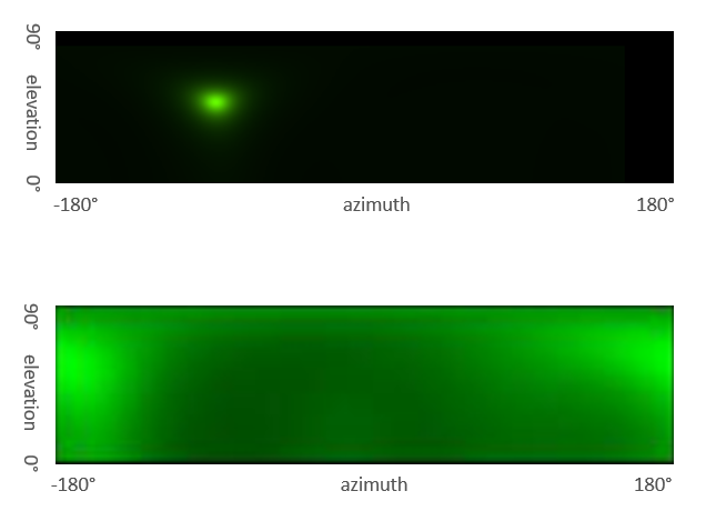
In an ideal case, MUSIC has excellent resolution in a good SNR environment and is very accurate. On the other hand, its performance is not very strong when the input signals are highly correlated, especially in an indoor environment. Multipath effects distort the pseudo-spectrum, causing it to have maximums at the wrong locations. The following figure compares the pseudospectrum under ideal circumstances (above) and in a real environment with a lot of reflections (below).
More information about the conventional beamformer and MUSIC estimators can be found in Z. Chen, G. Gokeda, Y. Yu, Introduction to Direction-of-Arrival Estimation, Artech House, 2010.
Spatial Smoothing#
Spatial smoothing is a method for solving problems caused by multipathing propagation when coherent signals are present. It can be proved that the signal covariance matrix can be "decorrelated" by calculating an averaged covariance matrix using subarrays of the original covariance matrix. For a two-dimensional array, this can be written as the following:

where 𝑀s and 𝑁s are the number of subarrays in x and y directions respectively and 𝑅𝑚n stands for the (𝑚, 𝑛)th sub array covariance matrix. An example proof of this formula and more information can be found in Y.-M. Chen, “On Spatial Smoothing for Two-Dimensional Direction-of-Arrival Estimation of Coherent Signals”, IEEE Transactions on Signal Processing, Vol. 45, No. 7, July 1997.
The resulting covariance matrix can now be used as a "decorrelated" version of the covariance matrix and fed to the MUSIC algorithm to produce correct results. The downside of spatial smoothing is that it reduces the size of the covariance matrix, which further reduces the accuracy of the estimate.
Challenges#
As shown earlier, calculating angle estimates in an ideal environment is insufficient. They must also be calculated in environments with heavy multipath effects, where signals are highly correlated or coherent. A coherent signal means a signal that is delayed and is a scaled version of some other signal. This can be the case when radio waves are reflected from walls, for example. Other challenges include signal polarization. In most cases, the polarization of the mobile device cannot be controlled, so the system has to take this into account. Also signal noise, clock jitter, and signal propagation delays add their own variables to the problem. Depending on the system scale, the RAM and especially CPU requirements can be demanding for an embedded system. Many of the effective angle estimation algorithms require a significant amount of processing power from the CPU.
A proper angle estimator algorithm must consider all these issues, and apply advanced techniques to reduce their adverse effects to the minimum.