Interpreting IQ Samples#

Sampling#

Although the Constant Tone Extension is a simple continuous wave – with a variable length of 16 μs to 160 μs – it is divided into periods as defined in the Bluetooth Core Specification (Vol. 6, Part B, Section 2.5).

The first 4 μs of the Constant Tone Extension is called the guard period and the next 8 μs is called the reference period. After the reference period, the Constant Tone Extension consists of a sequence of alternating switch slots and sample slots, each either 1 μs or 2 μs long, as specified by the application using the CTE Transmitter and CTE Receiver APIs. 2-μs slots make it possible to use a cheaper RF switch between the antennas that has a longer transition time. 1-μs slots make it possible to sample each antenna multiple times, which can help reduce the effect of noise and result in better accuracy.

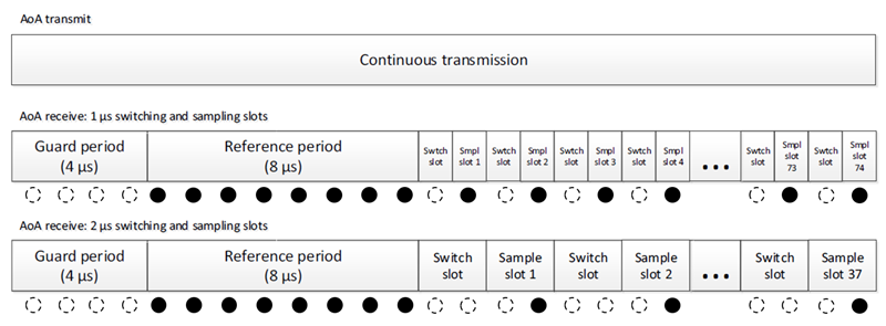
Once a CTE has started, the radio starts sampling the In-phase (I) and Quadrature (Q) components of the baseband signal with its native sample rate. The samples are then downsampled to 1 sample/μs sample rate. The first 4 samples (taken in the guard period) are discarded, then 8 samples (taken in the reference period) are stored in the sample buffer. Finally, every sample taken in switching slots is discarded and every sample taken in sample slots is stored in the sample buffer. In case of 2-μs slots, only one sample is kept for each sample slot. Stored samples are marked with filled circles on the previous figure.

At this point, N = 8 + (L – 12) / 2 / S number of samples are in both the In-phase (I) and in the Quadrature (Q) sample buffer, where L is the length of the CTE in microseconds, and S is the length of the slots in microseconds. The I and Q samples are merged into a common IQ sample buffer with 2N elements so that I and Q samples follow each other alternating:

I(0), Q(0), I(1), Q(1), I(2), Q(2), I(3), Q(3), … I(N), Q(N).

This IQ sample buffer is passed to the application for further processing.

Antenna Switching#

The goal of CTE is, to be able to sample the same continuous wave on different antennas. Since the radio can only sample on one antenna at a time, an RF path switching network must be created among the antennas, as shown in the following figure.

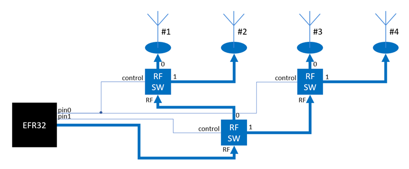
This way, any antenna can be connected with the EFR32 through control pins. The Bluetooth stack is designed so that it can drive up to six output pins to control the RF switches during CTE reception. With this solution up to 64 antennas can be addressed. As an example, on the previous image the four antennas can be addressed with the following addresses:

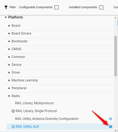
The six control pins can be selected in the configuration file of the Platform > Radio > RAIL Utility, AoX software component.

The antenna switching pattern, which is the order of addressing the different antennas, can be set with the CTE Receiver and CTE Transmitter Bluetooth APIs as described in the Bluetooth API Reference. For example, to set the antenna switching pattern for connectionless AoA mode, use the following code:

// Antenna switching pattern
static const uint8_t antenna_array[16] = { 0, 1, 2, 3, 4, 5, 6, 7, 8, 9, 10, 11, 12, 13, 14, 15 };

sl_bt_cte_receiver_enable_connectionless_cte(sync_handle,
                                             CTE_SLOT_DURATION,
                                             CTE_COUNT,
                                             sizeof(antenna_array),
                                             antenna_array);

The Bluetooth stack automatically controls the antenna switch pins in the switch slots of the CTE according to the defined switching pattern. The switching pattern can have any length between 1 and 35. It is repeated over the CTE time period, in other words once the end of the pattern is reached it starts over, and this is repeated until the end of the CTE signal. Note that the first switch happens after the reference period, which means that the first antenna in the pattern will be sampled 8 times.

Considering all of this, a switching pattern of [4 3 2 1] results in the following IQ samples:

where the indices mean the address of the antenna. Note, that the addresses do not necessarily have to be consecutive values starting from 0. Addresses can be any value between 0 and 63 and they should always be derived from the RF switching network.

Phase Retrieval#

IQ samples are passed to the application in a form of a uint8 array, with each I and Q sample taking 1-1 byte. Note, however, that I and Q samples are signed integers, which means that the uint8 values must be casted to int8 values immediately after the application receives them from the Bluetooth stack. Using uint8 values is simply a limitation of the BGAPI.

I and Q samples represent the in-phase and quadrature components of the signal, that is

s(t) = I(t) cos(2 π f t) + Q(t) sin(2 π f t),

where s(t) is the incoming signal, f is the carrier frequency and t is time. If the signal is phase-modulated (or frequency-modulated, which can be derived from phase modulation), it can be written in the following form:

s(t) = A cos(2 π f t + φ(t)) = A cos(2 π f t) cos( φ(t) ) – A sin(2 π f t) sin( φ(t) ),

where A is the amplitude of the signal and φ(t) is the instantaneous phase. From these equations the I and Q components of a phase modulated signal correspond to

I(t) = A cos( φ(t) ) and Q(t) = - A sin( φ(t) )

from which it is easy to retrieve the amplitude and the instantaneous phase of the signal:

Note that the amplitude does not represent the absolute amplitude of the signal, since it is compensated with AGC (automatic gain control). To learn the absolute amplitude of the signal, RSSI must be accounted for as well. Direction-finding algorithms do not usually need to do this, since all that matters is the phase difference and amplitude difference between antennas.

Phase Compensation#

Ideally, all antennas should be sampled at the same time to easily calculate the phase difference between them. However, this is not possible with a single radio. The only way to sample more than one antenna is time division, which also means that the sampling is shifted in time.

Note that, if antennas are not sampled at the same time, then even if φ(t) is constant and same for all antennas, there will be a phase increase of between two samples, where f is the carrier frequency and Δt is the time difference between two samples. Although the incoming signal is mixed and downsampled by the radio such that the central frequency of the channel corresponds to a DC signal in the baseband, the CTE will not have zero frequency in the baseband for two reasons:

• CTE is not using the central frequency. Instead it is generated as a sequence of continuous non-whitened 1’s, which corresponds to a continuous wave with the frequency of, where fc is the central frequency of the channel and fΔ is the frequency deviation. This corresponds to a frequency of fΔ in the baseband.

• Oscillators are not always perfectly tuned, which results in an offset between the ideal carrier frequency and the real carrier frequency. This again introduces a frequency shift foffset in the CTE frequency.

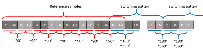
Considering this, the frequency of the CTE signal in the baseband is fΔ + foffset, where fΔ = 250kHz according to the Bluetooth specification, and foffset is in the order of 10kHz. Consequently, the phase shift between two consecutive samples with a 1-μs difference is around. Taking the offset frequency into account as well, it might vary between 80°-100°.

Since the reference samples are taken on the same antenna, they can be used to measure the actual phase shift over a 1-μs time period. It is strongly recommended to calculate the phase shift for each packet, as it may vary between packets. That is, every time an iq_report event is received, the first 8 IQ samples should be used to determine the phase shift for the actual packet. This can be done either by averaging the phase differences between the first 8 samples or by applying a median filter on those phase differences.

Note, however, that once a phase shift for 1 μs is calculated, this value should be multiplied and used to compensate for the phase shift between samples after the reference period due to the non-sampled switching slots, as illustrated in section Sampling. For 1-μs slots, 2 times the value should be used, and for 2-μs slots, 4 times the value should be used.

The content of the IQ sample buffer for a k-long antenna switching pattern is illustrated in the following figure along with the expected phase differences between the consecutive IQ samples, assuming that there is no phase shift between the antennas due to oblique angle of arrival.